Functional Connectivity Tutorial

Note

These examples were run on the ESI HPC cluster. This is why we use esi_cluster_setup() to set up a parallel computing client. They are perfectly reproducible on any other cluster or local machine by instead using slurm_cluster_setup() or local_cluster_setup() respectively.

The following Python code demonstrates how to use ACME to concurrently compute the functional connectivity in fMRI datasets of multiple subjects.

We start by downloading a publicly available fMRI dataset comprising BOLD signals from 33 adults using the Nilearn package:

from nilearn import datasets

data = datasets.fetch_development_fmri(age_group="adult")

The brain regions of interest (ROI) are taken from Power et al. 2011 comprising an atlas of 264 areas.

from nilearn import plotting

atlas = datasets.fetch_coords_power_2011(legacy_format=False)

Next, we extract ROI-averaged time-series from the downloaded fMRI data. To do this, we first use the MNI coordinates of every ROI in the atlas as seeds for masking the fMRI data:

from nilearn.maskers import NiftiSpheresMasker

atlasCoords = np.vstack((atlas.rois['x'],
                         atlas.rois['y'],
                         atlas.rois['z'])).T
masker = NiftiSpheresMasker(seeds=atlasCoords, smoothing_fwhm=6,
                            radius=5., detrend=True,
                            standardize=True,
                            low_pass=0.1, high_pass=0.01, t_r=2)

Next, we pick a random subject (Number 0) and perform the signal extraction removing nuisance regressors shipped with the fMRI dataset

timeseries = masker.fit_transform(data.func[0],
                                  confounds=data.confounds[0])

The extracted BOLD time-courses are contained in a (#time-points x #ROIs) = (168 x 264) array. We choose partial correlation as statistical dependence metric for computing the functional connectivity across all 264 regions in our atlas. Specifically, we compute the sparse inverse covariance matrix of the BOLD data with a cross-validated choice of the \(\ell^1\)-penalty using scikit-learn’s GraphicalLassoCV

from sklearn.covariance import GraphicalLassoCV

estimator = GraphicalLassoCV()
estimator.fit(timeseries)

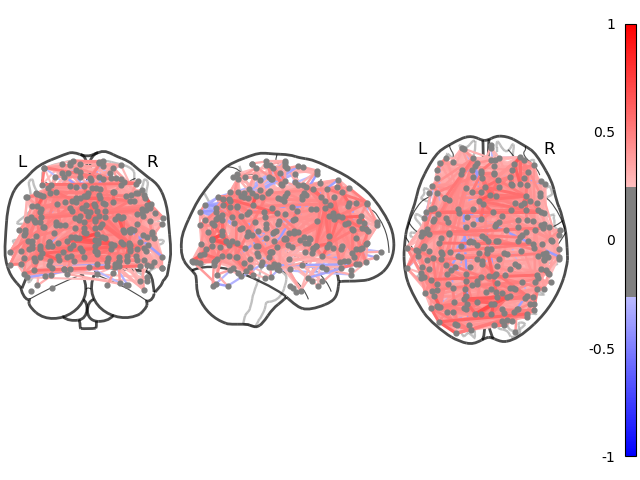
To visualize the computed inter-areal functional connectivity of Subject #0, we use Nilearns plot_connectome()

from nilearn import plotting

plotting.plot_connectome(estimator.covariance_, atlasCoords,
                         title=f"Subject #{subIdx}",
                         edge_threshold="95%", node_size=20,
                         colorbar=True, edge_vmin=-1, edge_vmax=1,
                         figure=fig)

Functional Connectivity in Parallel

In order to compute the functional connectome of multiple subjects concurrently, we first capsulate the computational steps in a Python function called compute_connectome which we define inside a dedicated module connectome.py:

import numpy as np
from nilearn import datasets
from nilearn.maskers import NiftiSpheresMasker
from sklearn.covariance import GraphicalLassoCV
from numpy.typing import NDArray

# Format atlas coordinates
atlas = datasets.fetch_coords_power_2011(legacy_format=False)
atlasCoords = np.vstack((atlas.rois['x'],
                         atlas.rois['y'],
                         atlas.rois['z'])).T

def compute_connectome(subidx : int) -> NDArray[np.float64]:
    """
    Compute functional connectome of single subject

    Parameters
    ----------
    subidx : int
        Subject number

    Returns
    -------
    con : 2D np.ndarray
        Functional connectivity matrix
    """

    # Take stock of data on disk
    data = datasets.fetch_development_fmri(age_group="adult")

    # Extract fMRI time-series averaged within spheres @ atlas coords
    masker = NiftiSpheresMasker(seeds=atlasCoords, smoothing_fwhm=6,
                                radius=5., detrend=True,
                                standardize=True, low_pass=0.1,
                                high_pass=0.01, t_r=2)
    timeseries = masker.fit_transform(data.func[subidx],
                                      confounds=data.confounds[subidx])

    # Compute functional connectivity b/w brain regions
    estimator = GraphicalLassoCV()
    estimator.fit(timeseries)
    return estimator.covariance_

We now define a set of subjects to analyze and set up a parallel computing client to do the actual processing

from connectome import compute_connectome
from acme import esi_cluster_setup, ParallelMap

subjectList = list(set(range(20)).difference([7, 8, 11, 12, 19]))
myClient = esi_cluster_setup(n_workers=8, mem_per_worker="8GB",
                             cores_per_worker=2, partition="E880")

The return value of compute_connectome is always a (#ROIs x #ROIs) = (264 x 264) matrix for all subjects. Thus, we want to store the computed functional connectivity matrices in a single shared 3d-array for easier post-processing. We use ParallelMap’s result_shape keyword for that:

with ParallelMap(compute_connectome,
                 subjectList,
                 result_shape=(264, 264, None)) as pmap:
    pmap.compute()

The resulting array can be accessed like any other HDF5 dataset, e.g., to visualize the inter-areal functional connectivity of Subject #4, we can use

import h5py

sub4 = h5py.File(pmap.results_container, "r")["result_3"][()]
plotting.plot_connectome(estimator.covariance_, atlasCoords,
                         title=f"Subject #{subIdx}",
                         edge_threshold="95%", node_size=20,
                         colorbar=True, edge_vmin=-1, edge_vmax=1,
                         figure=fig)

For more information about using result_shape and virtual HDF5 datasets, see Collect Results in Single Dataset